Climate change is here, it’s real, and it won’t be easy for humans to deal with. But few things are all good or all bad, and so it may be for climate change, at least with respect to environmental science and management.

A vast literature has accumulated in the past two or three decades in geosciences, environmental sciences, and ecology acknowledging the pervasive—and to some extent irreducible—roles of uncertainty and contingency. This does not make prediction impossible or unfeasible, but does change the context of prediction. We are obliged to not only acknowledge uncertainty, but also to frame prediction in terms of ranges or envelopes of probabilities and possibilities rather than single predicted outcomes. Think of hurricane track forecasts, which acknowledge a range of possible pathways, and that the uncertainty increases into the future.

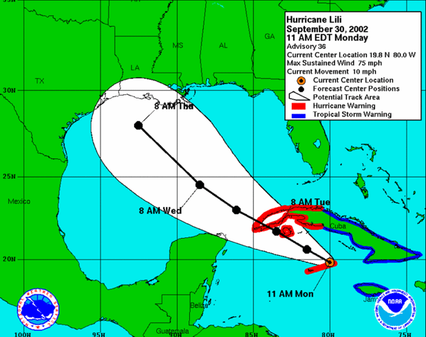
Forecast track for Hurricane Lili, September 30, 2002. The range of possible tracks and the increasing uncertainty over time are clear. Source: National Hurricane Center.

The foundation for time series analysis methods to detect chaos is the notion that phase spaces and dynamics of a nonlinear dynamical system (NDS) can be reconstructed from a single variable, based on Takens embedding theorem (Takens, 1981). Many years ago (Phillips, 1993) I showed that temporal-domain chaos in the presence of anything other than perfect spatial isotropy (and when does that ever happen in the real world?) leads to spatial-domain chaos. This implies an analogous principle in the spatial domain.

Assume an Earth surface system (ESS) characterized by n variables or components x_i, i = 1, 2, . . , n, which vary as functions of each other:

ESS = f(x₁, x_2, , , , x_n)

If spatial variation is directional along a gradient y (of e.g., elevation, moisture, insolation) then

dx_i/dy = f(x₁, x_2, , , , x_n)

dx₂/dy = f(x₁, x_2, , , , x_n)

.                 .                   .

.                 .                   .

.                 .                   .

Resistance of environmental systems is their capacity to withstand or absorb force or disturbance with minimal change. In many cases we can measure it based on, e.g., strength or absorptive capacity. Resilience is the ability of a system to recover after a disturbance or applied force to (or toward) its pre-disturbance condition—in many cases a function of dynamical stability. In my classes I illustrate the difference by comparing a steel bar and a rubber band. The steel bar has high resistance and low resilience—you have to apply a great deal of force to bend it, but once bent it stays bent. A rubber band has low resistance and high resilience—it is easily broken, but after any application of force short of the breaking point, it snaps back to its original state.

A couple of people (that is, about 50% of the blog’s readership) have asked about the “Jedi” reference in the Jedi Geoscience label. It comes from a PhD student about 10 years ago. After I answered his methodological question about his fieldwork, he good-naturedly suggested that my advice was about as helpful as if I had told him, like the Jedi Knights in the Star Wars movies, to “use the force.” After this story made the rounds, some of the grad students at Kentucky at the time referred to me as the “Jedi Geomorphologist.”

And now you know.

Jedi Geomorphologist using the force.

Some form of the diagram below is often used as a pedagogical tool, and to represent a theoretical framework, in fluvial geomorphology, hydrology, and river science. It is called a Lane Diagram, and originated in a publication by E.W. Lane in 1955:

The diagram shows that stream degradation (net erosion and incision) and aggradation (net deposition) responds to changes in the relationship between sediment supply (amount of sediment, Q_s, and typical sediment size, D₅₀) and sediment transport capacity (a function of discharge or flow, Q_w, and slope, S). The diagram is a very helpful metaphor in understanding the sediment supply vs. transport capacity relationship, and its effects on channel aggradation or degradation.

Nicholas Pinter, a Southern Illinois University geomorphologist, gave a nice talk yesterday on rivers and flooding in the 21^st century as part of UK’s Water Week. Pinter’s talk got me to thinking about the concept of “equilibrium” in environmental systems and what it means to both geoscientists and laypersons. Pinter correctly noted that rivers tend toward dynamic equilibrium, and more specifically, dynamic metastable equilibrium. This means three things: First, the system (river) is more or less constantly changing (the dynamic part). Second, equilibrium is of the type envisioned in mathematics and systems theory—that is, a state or condition the system settles into after a change or perturbation, with no further connotation other than that the response to the change has run its course (I’ve called this “relaxation time equilibrium” in my work). Third, “metastable” means that these equilibrium states are not necessarily stable and self-maintaining, and may be sensitive to future disturbances—even relatively small ones. Pinter’s message is that dynamic equilibrium in rivers means that rivers are constantly changing.